The post How to deploy object detection on Nvidia Jetson Nano appeared first on Ximilar: Visual AI for Business.
]]>What is NVIDIA Jetson Nano?
There were two reasons why using our API was not an option. First, the factory has unstable internet connectivity. Also, the entire solution needs to run in real time. So we chose to experiment with embedded hardware that can be deployed in such an environment, and we are very glad that we found Nvidia Jetson Nano.
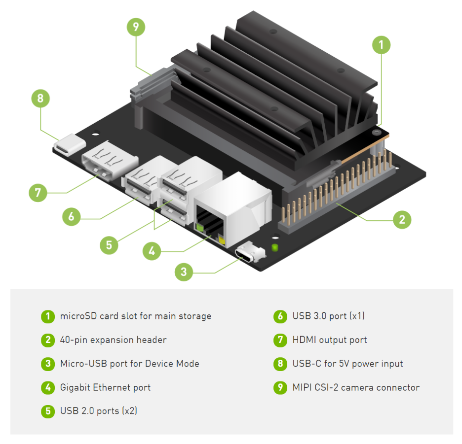
Jetson Nano is an amazing small computer (embedded or edge device) built for AI. It allows you to do machine learning in a very efficient way with low-power consumption (about 5 watts). It can be a part of IoT (Internet of Things) systems, running on Ubuntu & Linux, and is suitable for simple robotics or computer vision projects in factories. However, if you know that you will need to detect, recognize and track tens of different labels, choose the higher version of Jetson embedded hardware, such as Xavier. It is a much faster device than Nano and can solve more complex problems.
What is Jetson Nano good for?
Jetson is great if:
- You need a real-time analysis
- Your problem can be solved with one or two simple models
- You need a budget solution & be cost-effective when running the system
- You want to connect it to a static camera – for example, monitoring an assembly line
- The system cannot be connected to the internet – for example, because your factory is in a remote place or for security reasons
The biggest challenges in Africa & South Africa remain connectivity and accessibility. AI systems that can run in house and offline can have great potential in such environments.
Deloitte: Industry 4.0 – Is Africa ready for digital transformation?
Object Detection with Jetson Nano
If you need real-time object detection processing, use the Yolo-V4-Tiny model proposed in this repository AlexeyAB/darknet. And other more powerful architectures are available as well. Here is a table of what FPS you can expect when using Yolo-V4-Tiny on Jetson:
| Architecture | mAP @ 0.5 | FPS |
| yolov4-tiny-288 | 0.344 | 36.6 |
| yolov4-tiny-416 | 0.387 | 25.5 |
| yolov4-288 | 0.591 | 7.93 |
After the model’s training is completed, the next step is the conversion of the weights to the TensorRT runtime. TensorRT runtimes make a substantial difference in speed performance on Jetson Nano. So train the model with AlexeyAB/darknet and then convert it with tensorrt_demos repository. The conversion has multiple steps because you first convert darknet Yolo weights to ONNX and then convert to TensorRT.
There is always a trade-off between accuracy and speed. If you do not require a fast model, we also have a good experience with Centernet. Centernet can achieve a really nice mAP with precise boxes. If you run models with TensorFlow or PyTorch backends, then the speed is slower than Yolo models in our experience. Luckily, we can train both architectures and export them in a suitable format for Nvidia Jetson Nano.
Image Recognition on Jetson Nano
For any image categorization problem, I would recommend using simple architecture as MobileNetV2. You can select for example the depth multiplier for mobilenet of 0.35 and image resolution 128×128 pixels. In this way, you can achieve great performance both in speed and precision.
We recommend using TFLITE backend when deploying the recognition model on Jetson Nano. So train the model with the TensorFlow framework and then convert it to TFLITE. You can train recognition models with our platform without any coding for free. Just visit Ximilar App, where you can develop powerful image recognition models and download them for offline usage on Jetson Nano.
Recommended camera and utilities
Jetson Nano is simple but powerful hardware. However, it is not as powerful as your laptop or desktop computer. That’s why analyzing 4k images on Jetson will be very slow. I would recommend using max 1080p camera resolution. We used a camera by Raspberry PI, which works very well on Jetson and installation is easy!
I should mention that with Jetson Nano, you can come across some temperature issues. Jetson is normally shipped with a passive cooling system. However, if this small piece of hardware should be in the factory, and run stable for 24 hours, we recommend using an active cooling system like this one. Don’t forget to run the next command so your fan on Jetson starts working:
sudo jetson_clocks --fan
Installation steps & tips for development
When working with Jetson Nano, I recommend following guidelines by Nvidia, for example here is how to install the latest TensorFlow version. There is a great tool called jtop, which visualizes hardware stats as GPU frequency, temperature, memory size, and much more:
Remember, the Jetson has shared memory with GPU. You can easily run out of 4 GB when running the model and some programs alongside. If you want to save more than 0.5 GB of memory on Jetson, then run the Ubuntu on LXDE desktop environment/interface. The LXDE is more lightweight than the default Ubuntu environment. To increase memory, you can also create a swap file. But be aware that if your project requires a lot of memory, it can eventually destroy your microSD card. More great tips and hacks can be found on JetsonHacks page.
For improvement of the speed of Jetson, you can also try these two commands, which will set the maximum power input and frequency:
sudo nvpmodel -m0
sudo jetson_clocks
When using the latest image for Jetson, be sure that you are working with the right OpenCV versions of the library. For example, some older tracking algorithms like MOSSE or KCF from OpenCV require a specific version. For some tracking solutions, I recommend looking on PyImageSearch website.
Developing on Jetson Nano
The experience of programming challenging projects, exploring new gadgets, and helping our customers is something that deeply satisfies us. We are looking forward to trying other hardware for machine learning such as Coral from Google, Raspberry Pi, or Intel Movidius for Industry 4.0 projects.
Most of the time, we are developing a machine learning API for large e-commerce sites. We are really glad that our platform can also help us build machine learning models on devices running in distant parts of the world with no internet connectivity. I think that there are many more opportunities for similar projects in the future.
The post How to deploy object detection on Nvidia Jetson Nano appeared first on Ximilar: Visual AI for Business.
]]>The post OpenVINO: Start Optimizing Your TensorFlow 2 Models for Intel CPUs with Docker appeared first on Ximilar: Visual AI for Business.
]]>You can find extensive documentation on the official homepage, there is the GitHub page, some courses on Coursera and many other resources. But how to start as fast as possible without a need to study all of the materials? One of the possible ways can be found in the following paragraphs.
No Need to Install, Use Docker
OpenVINO has a couple of dependencies which need to be present on your computer. Additionally, to install some of them, you need to have root/admin rights. This might not be desirable. Using Docker represents much cleaner way. Especially when there is an image prepared for you on Docker Hub.
If you are not familiar with Docker, it might seem like a complicated piece of software, but we highly recommend you to try it and learn the basics. It is not hard and worth the effort. Docker is an important part of today’s SW development world. You will find installation instructions here.
Running the Docker Image
Containers are stateless. That means that next time you start your container, all the changes made will be gone. (Yes, this is a feature.) If you want to persist some files, just prepare a directory on your filesystem and we will bind it as a shared volume to a running container. (To /home/openvino
We will run our container in interactive mode (-it--rm
docker run -it --rm -v __YOUR_DIRECTORY__:/home/openvino openvino/ubuntu18_dev:latestTo be able to use all the tools, OpenVINO environment needs to be initialized. For some reason, this is not done automatically. (At least not for a normal user, if you start docker as a root, -u 0, setup script is run.)
source /opt/intel/openvino/bin/setupvars.shConformation is then printed out.
[setupvars.sh] OpenVINO environment initializedTensorFlow 2 Dependencies
TensorFlow 2 is not present inside the container by default. We could very easily create our own image based on the original one with TensorFlow 2 installed. This is the best way in production. With this being said, we will show you another way using the original container and installing the missing packages to an virtual environment into the shared directory (volume). This way, we can create as many such environments as we want. Or easily modify this environment. In addition, we will be still able to try the older TensorFlow 1 models. We prefer this approach during initial development.
Following code needs to be executed only once, after you first start your container.
mkdir ~/env
python3 -m venv ~/env/tensorflow2 --system-site-packages
source ~/env/tensorflow2/bin/activate
pip3 install --upgrade pip
pip3 install -r /opt/intel/openvino/deployment_tools/model_optimizer/requirements_tf2.txt
When you close your container and open it again, this is the only part you will need to repeat.
source ~/env/tensorflow2/bin/activateConverting TensorFlow SavedModel
Let’s say you have a trained model in SavedFormat. For the sake of this tutorial, we can take a pretrained MobileNet. Execute python3
import tensorflow as tf
model = tf.keras.applications.MobileNetV2(input_shape=(224,224,3))
model.save("/home/openvino/models/tf2")
Conversion is a matter of one command. However, there are few important parameters we need to use and which will be described below. Complete list can be found in the documentation. Exit python interpreter and run following command in a bash.
/opt/intel/openvino/deployment_tools/model_optimizer/mo_tf.py --saved_model_dir ~/models/tf2 --output_dir ~/models/converted --batch 1 --reverse_input_channels --mean_values [127.5,127.5,127.5] --scale_values [127.5,127.5,127.5]--batch 1--reverse_input_channels--mean_values [127.5,127.5,127.5] --scale_values [127.5,127.5,127.5]
Be careful, if you use pretrained models, different preprocessing and channel order can be used. If you try to use a neural network with input preprocessed in wrong way, you will of course get the wrong result.
You don’t need to include the preprocessing inside the converted model. The other option is to preprocess every image inside your own code before passing it to converted model. However, we use some OpenVINO inference tool which expects correct input.
At this point, we also need to mentioned that you might get slightly different values from SavedModel in TensorFlow and converted OpenVINO model. But from my experience on classification models, the difference is quite similar as when you use different ways to downscale your image to a proper input size.
Run Inference on Converted Model
First, we will get a testing picture which belongs to one of the 1000 ImageNet classes. We chose zebra, class index 340. (For TensorFlow, Google keeps the class indexes here.)
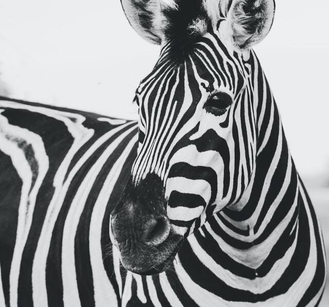
Let’s download it to our home directory We saved the small version of the image on our server so you can get it from there.
curl -o ~/zebra.jpg -s https://images.ximilar.com/tutorials/openvino/zebra.jpgThere is a script you can use for testing the prediction with no need to write any code.
python3 /opt/intel/openvino/deployment_tools/inference_engine/samples/python/classification_sample_async/classification_sample_async.py -i ~/zebra.jpg -m ~/models/converted/saved_model.xml -d CPUWe get some info lines and top 10 results at the end. Since the numbers are pretty clear, we will show only the first three.
classid probability
------- -----------
  340    0.9556126
  396    0.0032325
  721    0.0008250
Cool, our model is really sure about what is on the picture!
Using OpenVINO Inference in Python
That was easy, right? But you probably need to run the inference inside your own Python code. You can take a look inside the script. It is pretty straightforward, but for the sake of completeness, we will copy some of the code here. We will also add a code for running an inference on the original model so that you can compare it easily. If you please, run python3
We need one basic import from OpenVINO inference engine. Also, OpenCV and NumPy are needed for opening and preprocessing the image. If you prefer, TensorFlow could be used here as well of course. But since it is not needed for running the inference at all, we will not use it.
import cv2
import numpy as np
from openvino.inference_engine import IECore
As for the preprocessing, part of it is already present inside the converted model (scaling, changing mean, inverting input channels width and height), but that is not all. We need to make sure the image has a proper size (224 pixels both sides) and the dimensions are correct – batch, channel, width, height.
img = cv2.imread("/home/openvino/zebra.jpg")
img = cv2.resize(img, (224, 224))
img = np.expand_dims(img, 0)
img_openvino = img.transpose((0,3, 1, 2))
Now, we can try a simple OpenVINO prediction. We will use one synchronous request.
ie = IECore()
net = ie.read_network(model="/home/openvino/models/converted/saved_model.xml", weights="/home/openvino/models/converted/saved_model.bin")
input_name = next(iter(net.input_info))
output_name = next(iter(net.outputs))
net.batch_size = 1
# number of request can be specified by parameter num_requests, default 1
exec_net = ie.load_network(network=net, device_name="CPU")
# we have one request only, see num_requests above
request = exec_net.requests[0]
# infer() waits for the result
# for asynchronous processing check async_infer() and wait()
request.infer({input_name: img_openvino})
# read the result
prediction_openvino_blob = request.output_blobs[output_name]
prediction_openvino = prediction_openvino_blob.buffer
Our result, prediction_openvino
ids = np.argsort(prediction_openvino)[0][::-1][:3]
probabilities = np.sort(prediction_openvino)[0][::-1][:3]
for id, prob in zip(ids, probabilities):
    print(f"{id}\t{prob}")
We get exactly the same results as before. Our code works!
Comparing Results with Original TensorFlow Model
Now, let’s do the same with TensorFlow model. Do not forget to preprocess the image first. Prepared function preprocess_input can be used for that.
import tensorflow as tf
img_tf =  tf.keras.applications.mobilenet_v2.preprocess_input(img)
model = tf.keras.models.load_model("/home/openvino/models/tf2")
prediction_tf = model.predict(img_tf)
The results are almost the same, the difference is so small that we can ignore it. The top result from this prediction has probability 0.95860416, compared to 0.9556126 we had before. The order of the other predictions might be slightly different, because the values are so tiny.
By the way, there is a build-in function decode_predictions, which will not only give you the top results, but also class names and codes instead of just ids. Top 3 TensorFlow predictions.
from tensorflow.keras.applications.mobilenet_v2 import decode_predictions
top3 = decode_predictions(prediction_tf, top=3)
Here is the result:
[[('n02391049', 'zebra', 0.95860416), ('n02643566', 'lionfish', 0.0032956717), ('n01968897', 'chambered_nautilus', 0.0008273276)]]Benchmarking
We should mention that there is also a tool for benchmarking OpenVINO models called Benchmark Python Tool. It offers synchronous (latency-oriented) and asynchronous (throughput-oriented) measuring modes. Unfortunately, it does not work for other models (like TensorFlow) and cannot be used for direct comparison.
How OpenVINO Helped Us
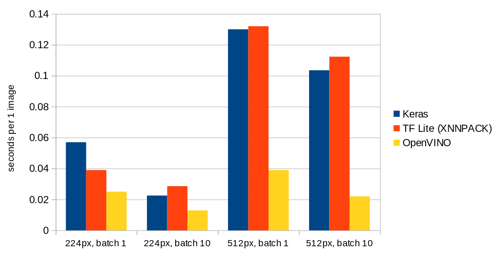
Enough of code, at the end of the article we will add some numbers. In Ximilar, we use often recognition models with resolution of 224 or 512 pixels. In a batch of 1 or 10. We used TensorFlow Lite format as often as possible, because it is very fast to load. (See a comparison here.) Because of a fast loading, it is not necessary to have the model in the cache all the time. To make running TF Lite models faster, we enhance the performance with XNNPACK.
Below you can see a chart with results for MobileNet V2. For the batches, we show prediction time in seconds per single image. Tests were done on our production workers.
Summary
In this article, we briefly introduced some of the basic functionality of OpenVINO. Of course, there is much more to try. We hope that this article has motivated you to try it yourself and maybe continue to explore all the possibilities through more advanced resources.
The post OpenVINO: Start Optimizing Your TensorFlow 2 Models for Intel CPUs with Docker appeared first on Ximilar: Visual AI for Business.
]]>The post How to Deploy Models to Mobile & IoT For Offline Use appeared first on Ximilar: Visual AI for Business.
]]>Earlier, in a separate blog post, we mentioned that one day you will be able to download your trained models offline. The time is now. We worked for several months with the newest TensorFlow 2+ (KUDOS to the TF team!), rewriting our internal system from scratch, so your trained models can finally be deployed offline.
Tadaaa — that makes Ximilar one of the first machine learning platform that allows its users to train a custom image recognition model with just a few clicks and download it for offline usage!
The feature is active only in custom pricing plans. If you would like to download and use your models offline, please let us know at sales@ximilar.com, where we are ready to discuss potential options with you.
Let’s get started!
Let’s have a look at how to use your trained model directly on your server, mobile phone, IoT device, or any other edge device. The downloaded model can be run on iOS devices, Android phones, Coral, NVIDIA Jetson, Raspberry Pi, and many others. This makes sense, especially in case your device is offline – if it’s connected to the internet, you can query our API to get results from your latest trained model.
Why offline usage?
Privacy, network connectivity, security, and high latency are common concerns that all customers have. Online use can also become a bottleneck when adopting machine learning on a very large scale or in factories for visual quality control. Here are some scenarios to consider offline models:
- You don’t want your data to leave your private network.
- Your device cannot be connected to the Internet or the connectivity is slow.
- You don’t need to request our API from your mobile for every image you make.
- You don’t want to be dependent on our infrastructure (but, BTW, we have almost 100% uptime).
- You need to do numerous queries (tens of millions) per day and want to run your models on your GPU cards.
Right now, both recognition models and detection models are ready for offline usage!
Before continuing with this article, you should already know how to create your Recognition models.
Download
After creating and training your Task, go to the Task page. Once you have permission to download the model, scroll down to the list of trained models and you should see the download icons. Choose the version of the model you are satisfied with and use the icon to download a ZIP file.
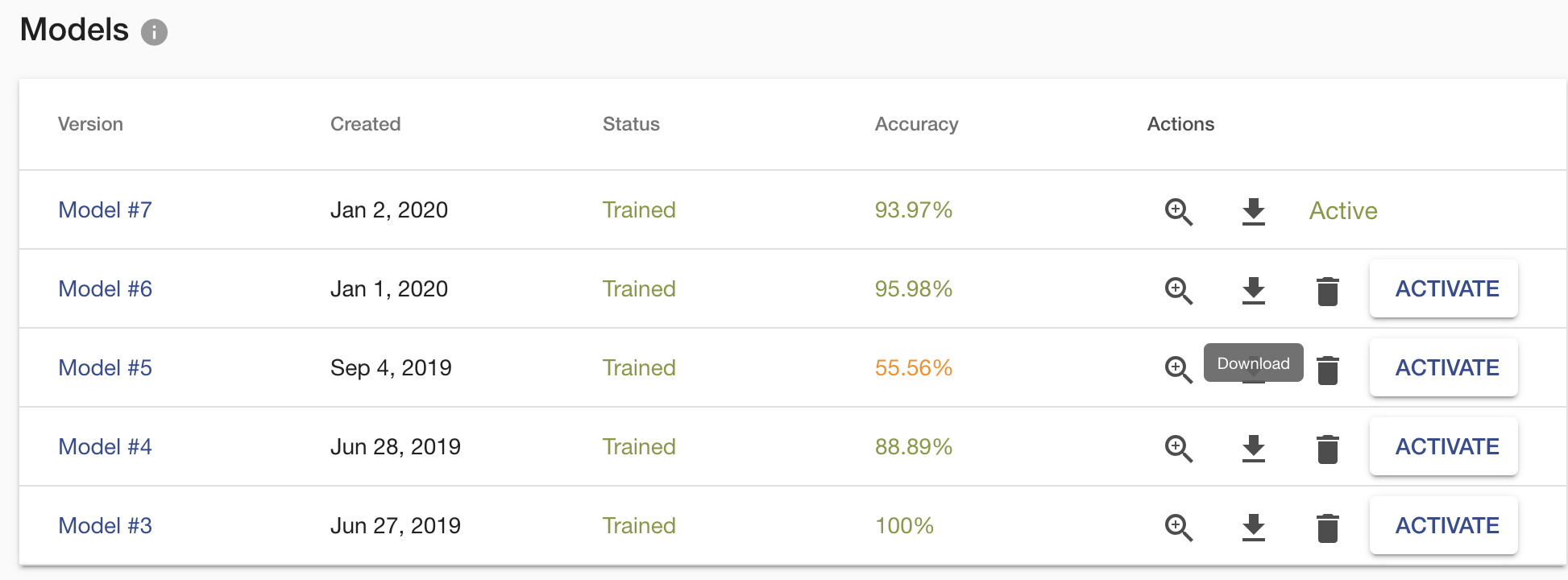
This ZIP archive contains several files. The actual model file is located in the tflite folder, and it is in TFLITE format which can be easily deployed on any edge device. Another essential file is labels.txt, which contains the names of your task labels. Order of the names is important as it corresponds with the order of model outputs, so don’t mix them up. The default input size of the model has a 224×224 resolution. There is another folder with saved_model which is used when deploying on server/pc with GPU.
Deploy on Android

That’s it!
Remember this is just a sample code on how to load the model and use it with your mobile camera. You can adjust/use code in a way you need.
Deploy on iOS
With iOS, you have two options. You can use either Objective-C or Swift language. See an example application for iOS. It is implemented in the Swift language. If you are a developer then I recommend being inspired by this file on GitHub. It loads and calls the model. The official quick start guide for iOS from the TensorFlow team is on tensorflow.org.
Workstation/PC/Server
If you want to deploy the recognition model on your server, then start with Ximilar-com/models repository. The folder scripts/recognition contains everything for the successful deployment of the model on your computer. You need to install TensorFlow with version 2.2+. If your workstation has an NVIDIA GPU, you can run the model on it. The GPU needs to have at least 4 GB of memory and CUDA Compute Capability 3.7+. Inferencing on GPU will increase the speed of prediction several times. You can play with the batch size of your samples, which we recommend when using GPU.
![]()
Edge and Embedded Devices
There is also the option to deploy on Coral, NVIDIA Jetson, or directly to a Web browser. Personally, we have a great experience on small projects with Jetson Nano. The MobilenetV2 architecture converted to TensorFlow LITE models works great. If you need to do object detection, tracking and counting then we recommend using YOLO architectures converted to TensorRT. YOLO can run on Jetson Nano in real-time settings and is fantastic for factories, assembly lines and conveyor belts with a small number of product types. You can easily buy and set up a camera on Jetson. Luckily, we are able to develop such models for you and your projects.
Update 2021/2022: We developed an object and image recognition system for Nvidia Jetson Nano for conveyor belts and factories. Read more at our blog post how to create visual AI system for Jetson.
Summary
Now you have another reason to use the Ximilar platform. Of course, by using offline models, you cannot use the Ximilar Flows which is able to connect your tasks to form a complex computer vision system. Otherwise, you can do with your model whatever you want.
To learn more about TFLITE format, see the tflite guide by the TensorFlow team. Big thanks to them!
If you would like to download your model for offline usage, then contact us at sales@ximilar.com and our sales team will discuss a suitable pricing model for you.
The post How to Deploy Models to Mobile & IoT For Offline Use appeared first on Ximilar: Visual AI for Business.
]]>